


Image Classification in Python: the Basics and a Quick Tutorial

Image classification is the task of assigning a label or class to an input image, based on its visual content. This is a common problem in computer vision and is used in a wide range of applications such as object recognition, facial recognition, and self-driving cars.
The process of image classification typically involves several steps:
- Pre-processing: This step involves preparing the input image for classification, which may include resizing, cropping, and normalizing the image.
- Feature extraction: This step involves extracting relevant features from the pre-processed image, which are then used as input to the classifier.
- Classification: This step involves using a machine learning model to make a prediction about the class of the input image, based on the extracted features.
There are various types of image classification, such as binary classification, multi-class classification, and multi-label classification. Deep learning models such as convolutional neural networks (CNNs) are commonly used for image classification due to their ability to automatically learn features from the input images.
Image classification using the Python programming language and libraries can be done using various machine learning techniques and libraries such as scikit-learn, TensorFlow, and Keras.
In This Article
Why Use Python for Image Classification?
Python is a popular choice for implementing image classification algorithms due to its simplicity, readability, and extensive library support.
Python has a number of libraries and frameworks that make it easy to implement image classification algorithms, including:
- NumPy: A library for working with large, multi-dimensional arrays and matrices of numerical data.
- SciPy: A library for scientific computing that provides functions for working with images, including reading and writing image files, resizing and cropping images, and applying image filters.
- scikit-learn: A machine learning library that provides a variety of algorithms for image classification, including support vector machines (SVMs) and decision trees.
- TensorFlow: A popular deep learning framework that provides a variety of tools for building and training neural networks for image classification tasks.
- PyTorch: Another popular deep learning framework that provides a variety of tools for building and training neural networks for image classification tasks.
These libraries and frameworks make it easy to implement image classification algorithms in Python, allowing developers to focus on the core logic of their algorithms rather than low-level implementation details.
The Importance of Data-Centric Approaches to Image Classification
Traditional computer vision models rely on model-driven AI, which focuses on building models that can simulate intelligent behavior. The emphasis is on designing and implementing models that can reason, plan, and make decisions based on a set of predefined rules or logic. This approach requires expert knowledge and domain-specific knowledge to simulate intelligent behavior.
A newer approach focuses on the data, rather than the model itself. Data-centric machine learning is important for image classification because the performance of an image classification model is heavily dependent on the quality and quantity of the training data. For example, the data inputs over time determine the accuracy of the model’s predictions, and are especially important to avoid degradation.
A data-centric approach may focus on the following:
- Quality: The training data should be representative of the types of images that the model will encounter in the real world. If the training data is not representative, the model will not perform well on new images. Additionally, the training data should be labeled correctly and accurately.
- Quantity: Generally, a model that is trained on a larger dataset performs better than one trained on a smaller dataset. This is especially true for deep learning models such as convolutional neural networks (CNNs), which have many parameters and require a large amount of data to train effectively.
- Data augmentation: This technique is used to artificially increase the size of the training data by applying random transformations to the images, or by using synthetic datasets. This can help to make the model more robust and reduce overfitting.
- Regularization: This technique is used to prevent overfitting by adding a term to the loss function that penalizes certain model parameters if they take on too large of a value.
Tutorial: Create Your Image Classification Model Using Python and Keras
This section is abbreviated from the image classification example provided in the Keras documentation. The example shows how to build an image classification model from scratch. You start with on-disk JPEG image files, and you don’t need to leverage a pre-built Keras model or pre-trained weights. This workflow uses Kaggle’s Cats vs. Dogs dataset for binary classification.
It uses image_dataset_from_directory to create a dataset, with Keras preprocessing layers enabling data augmentation and image standardization.
To set up Keras:
import tensorflow as tf
from tensorflow import keras
from tensorflow.keras import layers
Step 1: Load the Cats vs. Dogs dataset
Download the raw zip archive data:
!curl -O https://download.microsoft.com/download/3/E/1/3E1C3F21-ECDB-4869-8368-6DEBA77B919F/kagglecatsanddogs_5340.zip

!unzip -q kagglecatsanddogs_5340.zip
!ls
You should have an Animals folder containing two subfolders (Cats and Dogs):
!ls AnimalsSee the original example for an additional step to remove corrupted images.
Step 2: Create your dataset
To generate a new dataset use the following:
image_size = (180, 180)
batch_size = 128

train_ds, val_ds = tf.keras.utils.image_dataset_from_directory(
    "Animals",
    validation_split=0.2,
    subset="both",
    seed=1337,
    image_size=image_size,
    batch_size=batch_size,
)
Step 3: Visualize your data
The first nine images in your training dataset should appear as follows. Label 0 is Cat while label 1 is Dog:
import matplotlib.pyplot as plt

plt.figure(figsize=(10, 10))
for images, labels in train_ds.take(1):
    for i in range(9):
        ax = plt.subplot(3, 3, i + 1)
        plt.imshow(images[i].numpy().astype("uint8"))
        plt.title(int(labels[i]))
        plt.axis("off")
The output should look like this:
Corrupt JPEG data: 2226 extraneous bytes before marker 0xd4
Step 4: Augment the image data
If your dataset isn’t large enough, you can augment it artificially using random transformations to add realistic training image data. For example, you might use random small rotations or horizontal flipping to expose your model to a wider range or training aspects.
data_augmentation = keras.Sequential(
    [
        layers.RandomFlip("horizontal"),
        layers.RandomRotation(0.1),
    ]
)
You can visualize the augmented data samples by repeatedly applying the data_augmentation function to the first image in your dataset:
plt.figure(figsize=(10, 10))
for images, _ in train_ds.take(1):
    for i in range(9):
        augmented_images = data_augmentation(images)
        ax = plt.subplot(3, 3, i + 1)
        plt.imshow(augmented_images[0].numpy().astype("uint8"))
        plt.axis("off")
Step 5: Standardize the data
The images will be in the standard size of 240×240, with the dataset yielding them as float32 batches. However, having RGB channel values in range [0, 255] is not suitable for neural networks, so it is better to standardize them to keep the values in the range [0, 1]. You can do this with the rescaling layer.
Step 6: Preprocess your data
One way to use the data_augmentation preprocessor is to apply the preprocessor to your dataset. The resulting dataset should yield augmented image batches:
augmented_train_ds = train_ds.map(
    lambda x, y: (data_augmentation(x, training=True), y))
In this approach, data augmentation occurs asynchronously on the CPU, requiring buffering before it reaches the model. This option is better for CPU-based training because the data augmentation does not block the model. You should choose this approach when in doubt.
Step 7: Configure your dataset
The configuration should aim for optimal performance. Start by applying the data augmentation to your training dataset. Ensure that buffered prefetching is enabled to yield the data from disk while avoiding blocking. For example:
train_ds = train_ds.map(
    lambda img, label: (data_augmentation(img), label),
    num_parallel_calls=tf.data.AUTOTUNE,
)
train_ds = train_ds.prefetch(tf.data.AUTOTUNE)
val_ds = val_ds.prefetch(tf.data.AUTOTUNE)
Step 8: Build the model
In this example, we will build a small version of Xception. The architecture here isn’t optimized, but you can use KerasTuner to find the optimal model configuration. This process involves starting the model using data_augmentation and then the rescaling layer. A dropout layer should be included before the last fully connected layer:
def make_model(input_shape, num_classes):
    inputs = keras.Input(shape=input_shape)

    x = layers.Rescaling(1.0 / 255)(inputs)
    x = layers.Conv2D(128, 3, strides=2, padding="same")(x)
    x = layers.BatchNormalization()(x)
    x = layers.Activation("relu")(x)

    previous_block_activation = x

    for size in [256, 512, 728]:
        x = layers.Activation("relu")(x)
        x = layers.SeparableConv2D(size, 3, padding="same")(x)
        x = layers.BatchNormalization()(x)

        x = layers.Activation("relu")(x)
        x = layers.SeparableConv2D(size, 3, padding="same")(x)
        x = layers.BatchNormalization()(x)

        x = layers.MaxPooling2D(3, strides=2, padding="same")(x)

        residual = layers.Conv2D(size, 1, strides=2, padding="same")(
            previous_block_activation
        )
        x = layers.add([x, residual])
        previous_block_activation = x  # Set aside next residual

    x = layers.SeparableConv2D(1024, 3, padding="same")(x)
    x = layers.BatchNormalization()(x)
    x = layers.Activation("relu")(x)

    x = layers.GlobalAveragePooling2D()(x)
    if num_classes == 2:
        activation = "sigmoid"
        units = 1
    else:
        activation = "softmax"
        units = num_classes

    x = layers.Dropout(0.5)(x)
    outputs = layers.Dense(units, activation=activation)(x)
    return keras.Model(inputs, outputs)

model = make_model(input_shape=image_size + (3,), num_classes=2)
keras.utils.plot_model(model, show_shapes=True)
Step 9: Train the image classification model
Use the following script:
epochs = 25

callbacks = [
    keras.callbacks.ModelCheckpoint("save_at_{epoch}.keras"),
]
model.compile(
    optimizer=keras.optimizers.Adam(1e-3),
    loss="binary_crossentropy",
    metrics=["accuracy"],
)
model.fit(
    train_ds,
    epochs=epochs,
    callbacks=callbacks,
    validation_data=val_ds,
)
The validation accuracy should be high after training for 25 epochs (over 90%). Train for over 50 epochs will cause the degradation of the validation performance, a sign of overfitting.

Best Practices for Using Python for Image Classification
Here are some best practices for using Python for image classification:
- Use appropriate data types and structures: Use NumPy arrays and SciPy sparse matrices to represent images and other data structures in a way that is efficient and easy to manipulate.
- Preprocess and normalize your data: Before training your image classification model, it is important to preprocess and normalize your data. This can include tasks such as resizing images to a common size, converting images to grayscale, and applying image filters to remove noise. Normalizing your data can also help improve the performance of your model.
- Use a validation set to evaluate your model: When training a machine learning model, it is important to evaluate its performance on unseen data. This can be done by dividing your data into training and test sets and training your model on the training set and evaluating it on the test set. This can help you get a better sense of how your model will perform on real-world data.
- Use regularization to prevent overfitting: Overfitting occurs when a model is too complex and learns patterns in the training data that do not generalize to new, unseen data. One way to prevent overfitting is to use regularization, which involves adding constraints to the model to prevent it from becoming too complex.
- Use appropriate evaluation metrics: When evaluating the performance of your image classification model, it is important to use appropriate evaluation metrics. For example, if you are working with a balanced dataset (i.e., the same number of examples for each class), you can use metrics such as accuracy, precision, and recall. If you are working with an imbalanced dataset, you may want to use metrics such as the F1 score or AUC (Area Under the Curve).
Read More
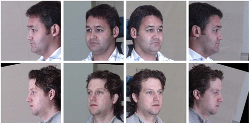
The State of Facial Recognition Today
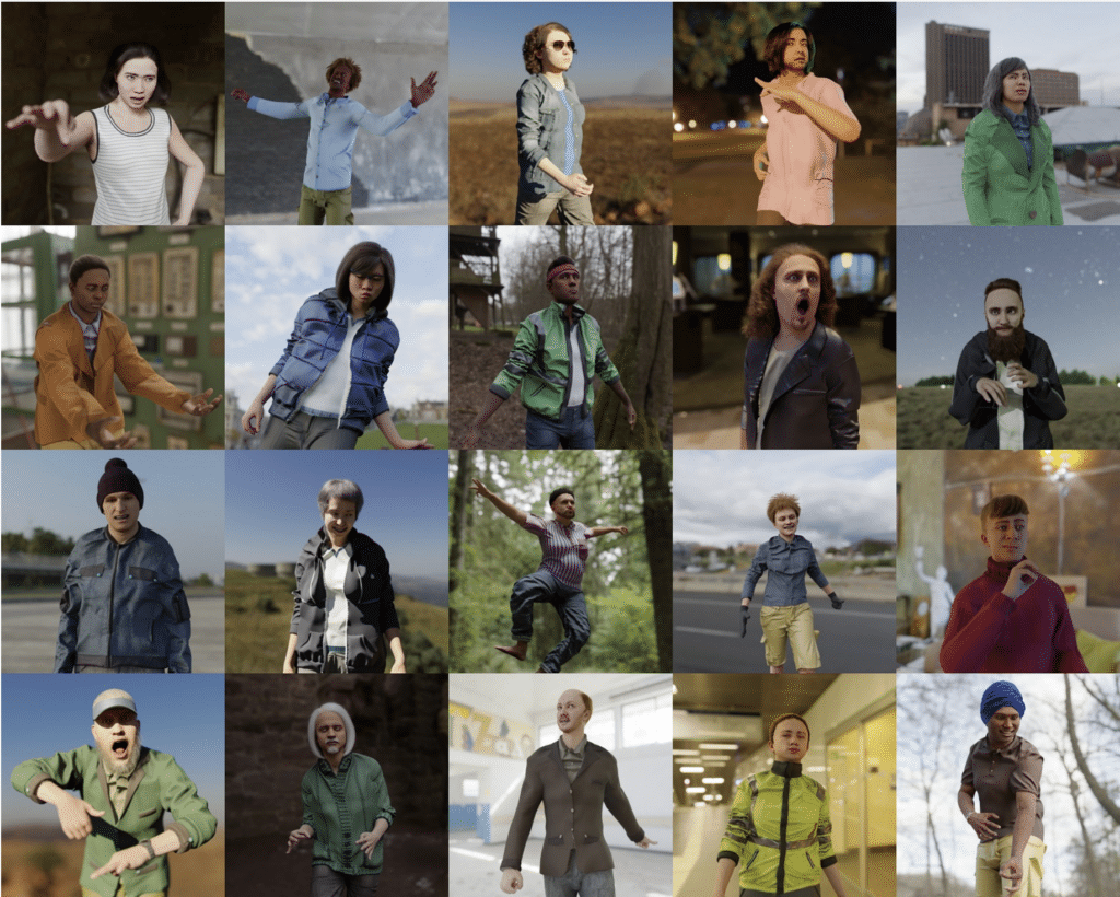
Procedural Humans for Computer Vision