


Image Classification Using CNN: Introduction and Tutorial

In This Article
How Are Convolutional Neural Networks (CNNs) Used for Image Classification?
Image classification is the task of assigning a label or class to an input image. It is a supervised learning problem, where a model is trained on a labeled dataset of images and their corresponding class labels, and then used to predict the class label of new, unseen images.
There are many architectures for image classification, one of the most popular being convolutional neural networks (CNNs). CNNs are especially effective at image classification because they are able to automatically learn the spatial hierarchies of features, such as edges, textures, and shapes, which are important for recognizing objects in images.
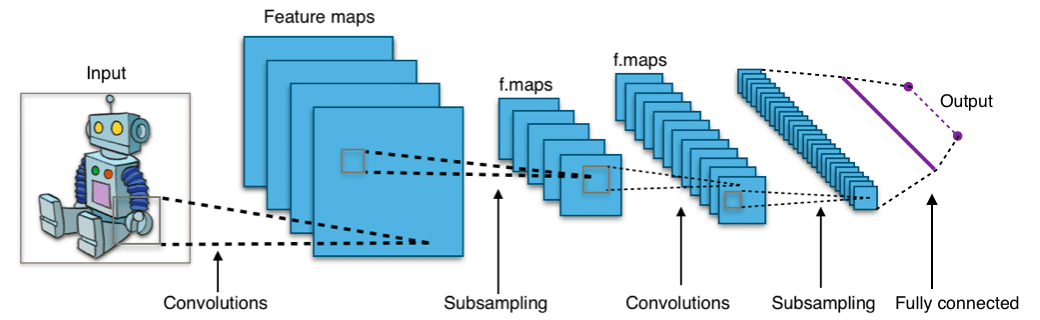
Image source: Wikimedia Commons
In a neural network, the layers comprise interconnected nodes or neurons that process the input data and pass it through the network to produce an output:
- The input layer is the first layer in the network and it is where the input data is fed into the network. The input layer does not perform any computation, it simply receives the input and passes it on to the next layer.
- The hidden layers are the layers that come after the input layer and before the output layer. These layers perform the bulk of the computation in the network, such as feature extraction and abstraction.
- The output layer is the final layer in the network and it produces the output of the network.
CNN for Image Classification: How It Works
CNNs consist of a series of interconnected layers that process the input data. The first hidden layer of a CNN is usually a convolutional layer, which applies a set of filters to the input data to detect specific patterns. Each filter generates a feature map by sliding over the input data and performing element-wise multiplication with the entries in the filter. These feature maps are then combined and passed through non-linear activation functions, such as the ReLU function, which introduces non-linearities into the model and allows it to learn more complex patterns in the data.
Subsequent layers in a CNN may include additional convolutional layers, pooling layers, and fully-connected layers. Pooling layers reduce the size of the feature maps. This helps reduce the overall number of parameters in the model and makes it more computationally efficient. Fully-connected layers are typically found after convolutional and pooling layers of a CNN. A fully-connected layer connects all the neurons in a layer to all the neurons in the next layer, allowing the model to learn possible non-linear combinations of the features learned by the convolutional layers.
The final layer of a CNN is typically a softmax layer, which produces a probability distribution across the possible class labels for the input data. The class that has the highest probability is chosen as the prediction of the model.
A few key points to understand about CNNs for classification:
- CNNs can learn to recognize patterns and features in images through the use of convolutional layers, which apply a set of filters to the input data to detect specific patterns.
- CNNs are able to automatically learn spatial hierarchies of features, starting with simple patterns such as edges and moving on to more complex patterns as the layers get deeper. This hierarchical feature learning is particularly well-suited to image classification, where the visual features of an image can vary widely.
- Some CNN architectures are able to process images in real-time, making them suitable for applications where quick classification is important, such as in self-driving cars or security systems.
- CNNs have achieved state-of-the-art performance on many image classification benchmarks and are widely used in industry and research.
Tutorial: CNN Image Classification with Keras and CIFAR-10
Here is a tutorial on how to perform image classification using a convolutional neural network (CNN) and the Keras library. You can find the code in this Google Colab notebook.
Step 1: Choose a Dataset
The first step is to choose a dataset for the image classification task. There are many publicly available datasets, such as CIFAR-10, CIFAR-100, and MNIST, that can be used for training and testing the CNN. For this tutorial, we will be using the CIFAR-10 dataset, which consists of 60,000 32×32 color images across ten classes, with 6,000 images in each class.
import tensorflow as tf
from tensorflow.keras import datasets
from tensorflow.keras.models import Sequential
from tensorflow.keras import layers
Step 2: Prepare the Dataset for Training
Next, we will load the CIFAR-10 dataset and prepare it for training. This involves splitting the dataset into training and test sets, and then normalizing the pixel values of the images to the range of 0 to 1.
# Download the data set
(train_images, train_labels), (test_images, test_labels) = datasets.cifar10.load_data()

train_images, test_images = train_images / 255.0, test_images / 255.0
Step 3: Create Training Data and Assign Labels
We will use the training set of images and labels to train the CNN. We will use the flow_from_directory() method from the keras.preprocessing.image module to create a generator that will read the images from the directory and apply data augmentation.
We will assign labels to the data by converting the categorical class labels to one-hot encoded vectors.
class_names = ['airplane', 'automobile', 'bird', 'cat', 'deer',
               'dog', 'frog', 'horse', 'ship', 'truck']
Step 4: Define and Train the CNN Model
We will define the CNN architecture using the Keras library. The model will consist of several convolutional layers followed by max pooling layers, and a fully connected layer with a softmax activation function. We will then train the model using the fit() method.
model = models.Sequential()
model.add(layers.Conv2D(32, (3, 3), activation='relu', input_shape=(32, 32, 3)))
model.add(layers.MaxPooling2D((2, 2)))
model.add(layers.Conv2D(64, (3, 3), activation='relu'))
model.add(layers.MaxPooling2D((2, 2)))
model.add(layers.Conv2D(64, (3, 3), activation='relu'))
model.add(layers.Flatten())
model.add(layers.Dense(64, activation='relu'))
model.add(layers.Dense(10))
model.compile(optimizer='adam',
loss=tf.keras.losses.SparseCategoricalCrossentropy(from_logits=True),
metrics=['accuracy'])
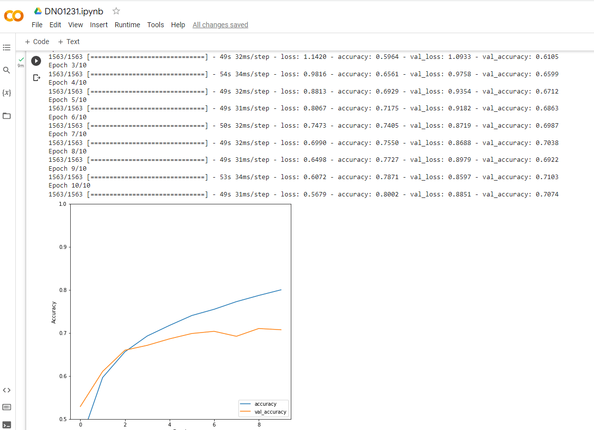
history = model.fit(train_images, train_labels, epochs=10,
validation_data=(test_images, test_labels))Step 5: Test the Model’s Accuracy
Finally, we will evaluate the trained model on the test set using the evaluate() method and calculate the accuracy of the model.
plt.figure(figsize=(8, 8))
plt.plot(history.history['accuracy'], label='accuracy')
plt.plot(history.history['val_accuracy'], label = 'val_accuracy')
plt.xlabel('Epoch')
plt.ylabel('Accuracy')
plt.ylim([0.5, 1])
plt.legend(loc='lower right')

plt.savefig("output_report.png")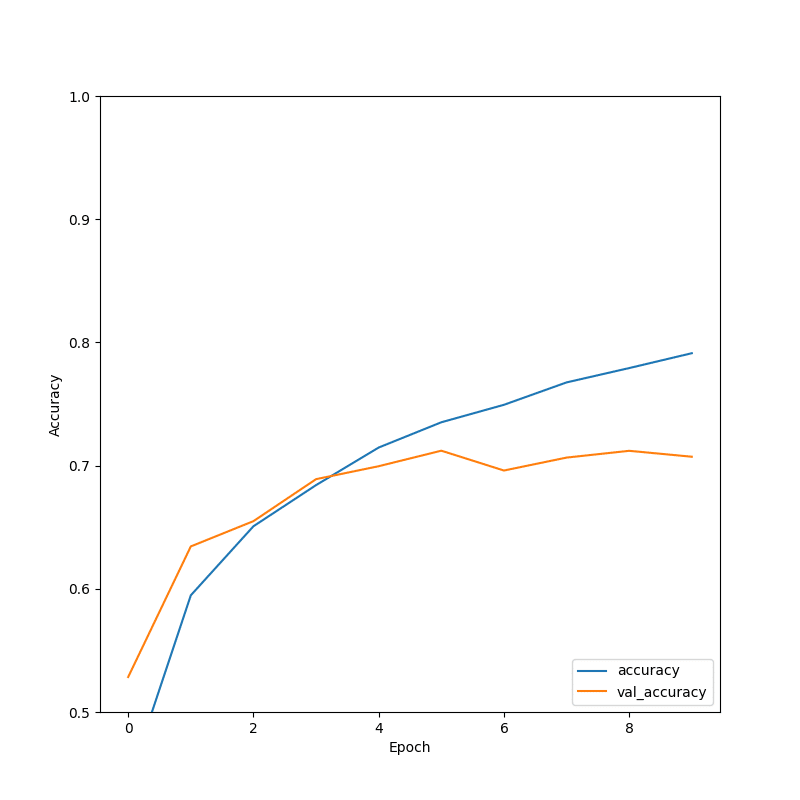
Read More
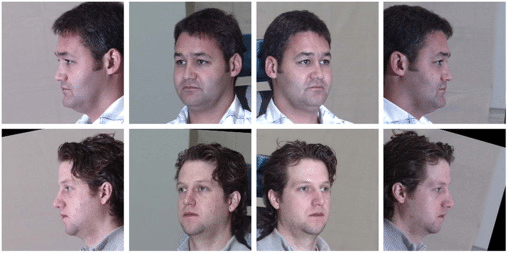
The State of Facial Recognition Today
Procedural Humans for Computer Vision