


Procedural Modeling: a brief introduction
One of the key challenges in the field of computer vision is assembling large enough datasets with enough variance. As we have explored in previous posts, the lack of high-quality labeled training data is a major bottleneck in the nascent field of computer vision.
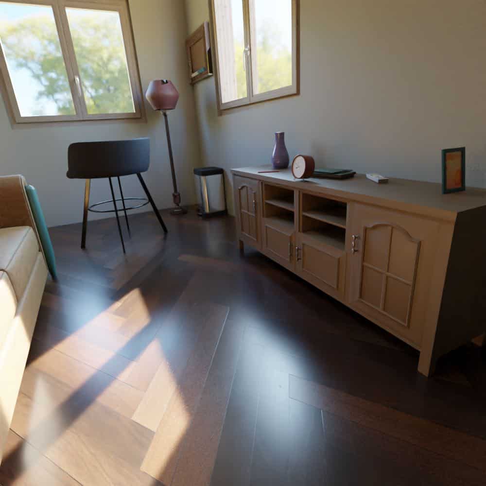
The complexity of image recognition and detection is compounded when objects are placed in realistic settings. In indoor environments, there is a huge range of variability that needs to be considered. Different furniture, layouts, and decor can present significant challenges for computer vision applications in indoor environments. Training a household robot on one image of a table or one image of a couch won’t suffice to effectively train it for different environments. The more variance in the dataset used to train the model, the more effective it will be.
Simulated Data solves this problem through algorithms that can create environments that contain the optimal diversity of objects that can be difficult to capture manually. But, in order to do so, our algorithms must be able to query from libraries of millions of unique 3D assets, representing the full diversity of our environments.
This has been challenging in the past because building a 3D asset library has relied on either scanning real objects one-by-one or modeling them from scratch. The expense and time associated with modeling the large number of assets needed for such a dataset has been prohibitive, limiting the technology’s ability to fully deliver on its potential.
At Datagen, we have developed exciting new technologies and pipelines to efficiently and effectively generate entire libraries of visual assets. The solution we use to solve this problem is called Procedural Modeling. Procedural Modeling is a technique that enables us to vary and change existing models based on a sequence of rules, instructions, or algorithms instead of creating entirely new ones. It consists of two main stages: Modular Modeling and Auto-Variation Modeling. Combining these two processes gives us the maximum number of variants, with minimum time and expense.
Modular and Auto-Variation Modeling
At its core, the goal of Procedural Modeling is to create the largest number of unique assets with the least amount of manual modeling work. To understand Procedural Modeling and the role it plays in Simulated Data, let’s explore its two different stages. We’ll use the process of modeling a 3D table as an example.
Watch on-demand “Implementing Data-Centric Methodology with Synthetic Data” with Meta and Microsoft
1. Modular Modeling
This first stage is to divide the object into separate physical components or modules. Let’s examine this table. We have two distinct components: the legs, and the table top. (You can imagine that more complex objects have a larger number of distinct parts.) In this stage, we treat each model as a separate object to be modeled independently. Logically, mixing and matching these components is one way to create unique assets – straight legs with a round table top vs. straight legs with a square table top vs. curved legs with a round table top. You can start to see how, with more modular variations you can start to create a larger number of unique variations. So, we model a number of variations of each module for the object.
2. Auto-Variation Modeling
But, we know that tables don’t just differ by the shape of the table top or the legs. Table tops can be bigger or smaller, round or oval; legs can be longer or shorter, more curved or straighter. A huge number of additional unique combinations can be obtained by changing not just the modular components, but the shapes and dimensions of each modular component itself.
Since 3D models are built of polygons and lines that connect points, we can manipulate the shape of the object by moving these points automatically and systematically. We just need to define key parameters that place bounds on length, height, and width and maintain the underlying geometry and structure. Make the legs longer, the surface wider or more square – and change all of these axes simultaneously. The table can elongate, and decrease in height, and then shorten and grow in height. We can capture each of these iterations of the table, sampling continuously, giving us a huge amount of variants. While programmatically manipulating all of these variables at once, we change the shape of the object and can save each iteration of the shape as something we call “Shape Keys.”
Add in variations in the materials – wood, metal, painted, etc. – and we start to have a huge library based on just limited numbers of modular components. So, while this approach still requires manual modeling of modular components, every modular variation you add in the first step, variation increases substantially in step two. And, automated generation pipelines allow for seamless conversions of shape keys into usable assets that can be sampled from our library. Compared to the manual method of building model after model after model, it’s clear how much faster and efficient procedural modeling is.
Different applications of computer vision require images and video of different objects and assets to train them to serve their purpose. However, they all need large datasets with enough variants of the right asset to effectively train them. Procedural Modeling is a powerful tool that enables us to achieve this.
Watch on-demand “Implementing Data-Centric Methodology with Synthetic Data” with Meta and Microsoft
Read More
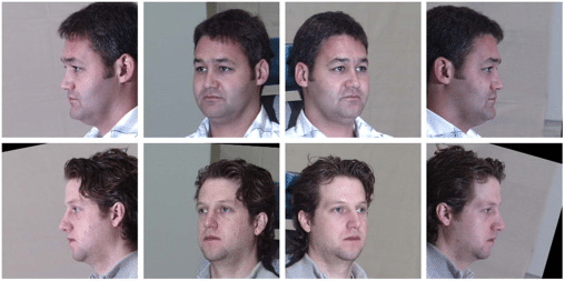
The State of Facial Recognition Today
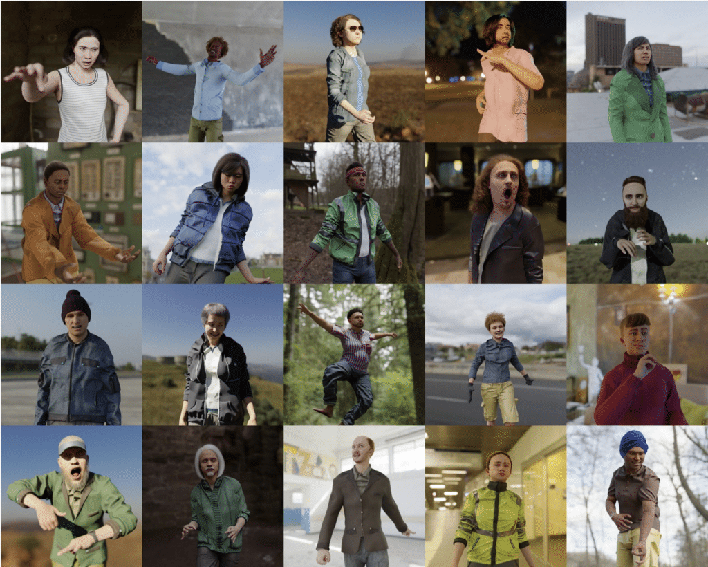
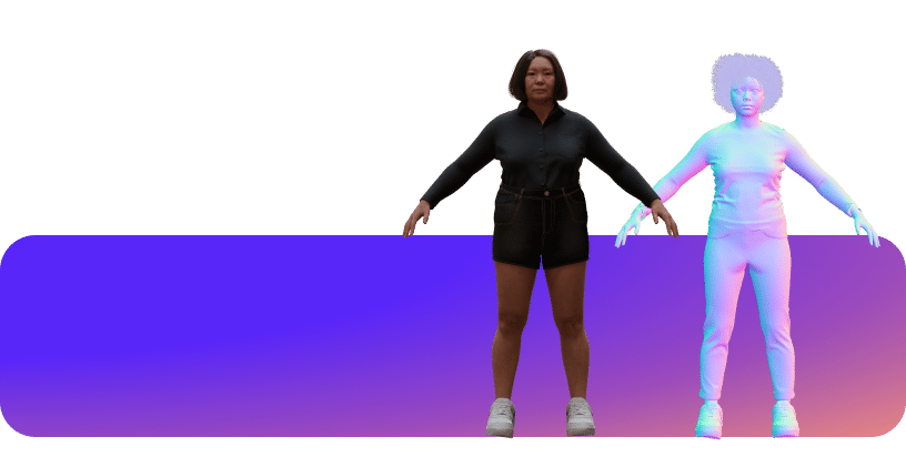
Procedural Humans for Computer Vision