


ResNet-50: The Basics and a Quick Tutorial
What Is the ResNet-50 Model?
ResNet stands for Residual Network and is a specific type of convolutional neural network (CNN) introduced in the 2015 paper “Deep Residual Learning for Image Recognition” by He Kaiming, Zhang Xiangyu, Ren Shaoqing, and Sun Jian. CNNs are commonly used to power computer vision applications.
ResNet-50 is a 50-layer convolutional neural network (48 convolutional layers, one MaxPool layer, and one average pool layer). Residual neural networks are a type of artificial neural network (ANN) that forms networks by stacking residual blocks.
In This Article
ResNet-50 Architecture
The original ResNet architecture was ResNet-34, which comprised 34 weighted layers. It provided a novel way to add more convolutional layers to a CNN, without running into the vanishing gradient problem, using the concept of shortcut connections. A shortcut connection “skips over” some layers, converting a regular network to a residual network.
The regular network was based on the VGG neural networks (VGG-16 and VGG-19)—each convolutional network had a 3×3 filter. However, a ResNet has fewer filters and is less complex than a VGGNet. A 34-layer ResNet can achieve a performance of 3.6 billion FLOPs, and a smaller 18-layer ResNet can achieve 1.8 billion FLOPs, which is significantly faster than a VGG-19 Network with 19.6 billion FLOPs (read more in the ResNet paper, He et, al, 2015).
The ResNet architecture follows two basic design rules. First, the number of filters in each layer is the same depending on the size of the output feature map. Second, if the feature map’s size is halved, it has double the number of filters to maintain the time complexity of each layer.
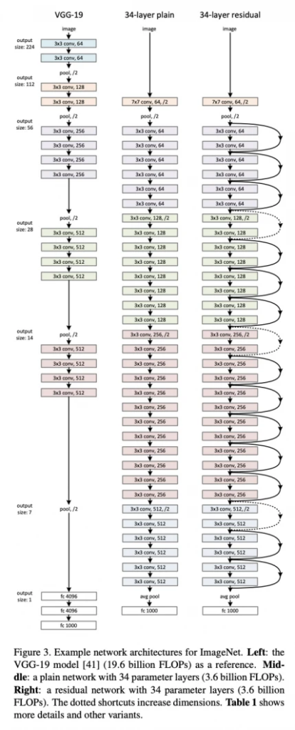
Source for this and the following images: Kaiming at al, Arxiv.org
Special characteristics of ResNet-50
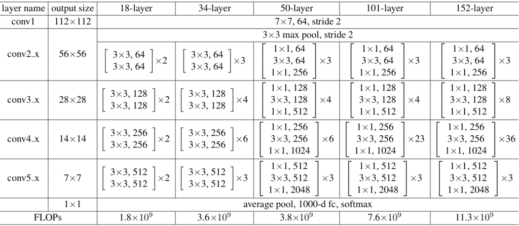
ResNet-50 has an architecture based on the model depicted above, but with one important difference. The 50-layer ResNet uses a bottleneck design for the building block. A bottleneck residual block uses 1×1 convolutions, known as a “bottleneck”, which reduces the number of parameters and matrix multiplications. This enables much faster training of each layer. It uses a stack of three layers rather than two layers.
The 50-layer ResNet architecture includes the following elements, as shown in the table below:
- A 7×7 kernel convolution alongside 64 other kernels with a 2-sized stride.
- A max pooling layer with a 2-sized stride.
- 9 more layers—3×3,64 kernel convolution, another with 1×1,64 kernels, and a third with 1×1,256 kernels. These 3 layers are repeated 3 times.
- 12 more layers with 1×1,128 kernels, 3×3,128 kernels, and 1×1,512 kernels, iterated 4 times.
- 18 more layers with 1×1,256 cores, and 2 cores 3×3,256 and 1×1,1024, iterated 6 times.
- 9 more layers with 1×1,512 cores, 3×3,512 cores, and 1×1,2048 cores iterated 3 times.
(up to this point the network has 50 layers)
- Average pooling, followed by a fully connected layer with 1000 nodes, using the softmax activation function.

Tutorial: ResNet-50 Transfer Learning with Keras
Transfer learning means taking a pre-trained machine learning model and repurposing it for another related task for faster development. It helps achieve higher performance even if the model is trained on a smaller dataset.
Import Required Libraries and Dataset
This tutorial implements a Restnet-50 model to use transfer learning and solve TensorFlow’s demo image classification problem. It will build a classifier to classify the dataset’s five different classes of flowers.
To import the required libraries and dataset for the problem:
1. Use the following commands to download the relevant libraries:
import matplotlib.pyplot as plotter_lib
import numpy as np
import PIL as image_lib
import tensorflow as tflow
from tensorflow.keras.layers import Flatten
from keras.layers.core import Dense
from tensorflow.keras.models import Sequential
from tensorflow.keras.optimizers import Adam
Note: to use PIL library you will need to install Pillow. You can install it using pip install Pillow
2. Use the following command to import that dataset for the problem:
import pathlib
demo_dataset = "https://storage.googleapis.com/download.tensorflow.org/example_images/flower_photos.tgz"
directory = tflow.keras.utils.get_file('flower_photos', origin=demo_dataset, untar=True)
data_directory = pathlib.Path(directory)
Partition and Visualize Data
The dataset needs to be split into two parts: one for training and one for validation. As each epoch passes, the model gets trained on the training subset. Then, it assesses its performance and accuracy on the validation subset simultaneously.
To split the data into two parts:
- Use the following command to create the training subset:
img_height,img_width=180,180
batch_size=32
train_ds = tflow.keras.preprocessing.image_dataset_from_directory(
data_directory,
validation_split=0.2,
subset="training",
seed=123,
label_mode='categorical',
image_size=(img_height, img_width),
batch_size=batch_size)
The above commands specify the images to have a 180×180 size. The validation_split parameter specifies 20% of the dataset for validation and the remaining for training. Users can tweak the batch_size parameter to suit the memory specifications of the machine.
2. Use the following command to create the validation subset:
validation_ds = tflow.keras.preprocessing.image_dataset_from_directory(
data_directory,
validation_split=0.2,
subset="validation",
seed=123,
label_mode='categorical',
image_size=(img_height, img_width),
batch_size=batch_size)
To import the pre-trained machine learning model:
Use the following command to visualize six random images from the dataset:
import matplotlib.pyplot as plotter_lib
plotter_lib.figure(figsize=(10, 10))
epochs=10
for images, labels in train_ds.take(1):
for var in range(6):
ax = plt.subplot(3, 3, var + 1)
plotter_lib.imshow(images[var].numpy().astype("uint8"))
plotter_lib.axis("off")*
Import the Pre-trained Model
The keras library comes with many cutting-edge machine learning algorithms that users can choose to solve a problem. This tutorial selects the ResNet-50 model to use transfer learning and create a classifier.
To import the ResNet-50 model from the keras library:
- Use the following code to import the model:
demo_resnet_model = Sequential()
pretrained_model_for_demo= tflow.keras.applications.ResNet50(include_top=False,
input_shape=(180,180,3),
pooling='avg',classes=5,
weights='imagenet')
for each_layer in pretrained_model_for_demo.layers:
each_layer.trainable=False
demo_resnet_model.add(pretrained_model_for_demo)
Setting include_top to False means it will allow adding input and output layers custom to a problem. The weights parameter specifies that the model uses its weights while training on the imagenet dataset. The for loop on the model’s layers ensures it doesn’t learn its weights again and saves on time and space.
2. Use the following commands to add a fully connected output layer to the model where the learning can happen:
demo_resnet_model.add(Flatten())
demo_resnet_model.add(Dense(512, activation='relu'))
demo_resnet_model.add(Dense(5, activation='softmax'))
The above code uses the softmax function and creates five neurons to classify the five flower classes in the dataset.
Train and Evaluate Model
To train the ResNet-50 model:
Use the following command to train the model on the training dataset:
demo_resnet_model.compile(optimizer=Adam(lr=0.001),loss='categorical_crossentropy',metrics=['accuracy'])
history = demo_resnet_model.fit(train_ds, validation_data=validation_ds, epochs=epochs)
To evaluate the ResNet-50 model after training the model:
Use the following command to evaluate the model and visualize the model’s training and accuracy changing with each epoch:
plotter_lib.figure(figsize=(8, 8))
epochs_range= range(epochs)
plotter_lib.plot( epochs_range, history.history['accuracy'], label="Training Accuracy")
plotter_lib.plot(epochs_range, history.history['val_accuracy'], label="Validation Accuracy")
plotter_lib.axis(ymin=0.4,ymax=1)
plotter_lib.grid()
plotter_lib.title('Model Accuracy')
plotter_lib.ylabel('Accuracy')
plotter_lib.xlabel('Epochs')
plotter_lib.legend(['train', 'validation'])
#If you are using Windows or Linux Desktop please uncomment following line. This will not work on command line/terminal based OS
#plotter_lib.show()
plotter_lib.savefig('output-plot.png') 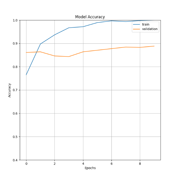
Model Inference
Before running the model on the dataset, the images must go through preprocessing steps. These steps ensure that each image’s dimensions correspond to what the model trained on.
To use the model and classify images:
- Use the following command to run the predictions on a sample image of a rose from the dataset:
import cv2
sample_image=cv2.imread(str(roses[0]))
sample_image_resized= cv2.resize(sample_image, (img_height,img_width))
sample_image=np.expand_dims(sample_image_resized,axis=0)
These commands use the OpenCV library for preprocessing.
2. Use the following command to make predictions:
image_pred=resnet_model.predict(image)
The above command prints an array of five numbers since the output layer uses softmax classifier.
3. Use the following command to produce a human-readable output label:
image_output_class=class_names[np.argmax(image_pred)]
print("The predicted class is", image_output_class)
Read More
The State of Facial Recognition Today
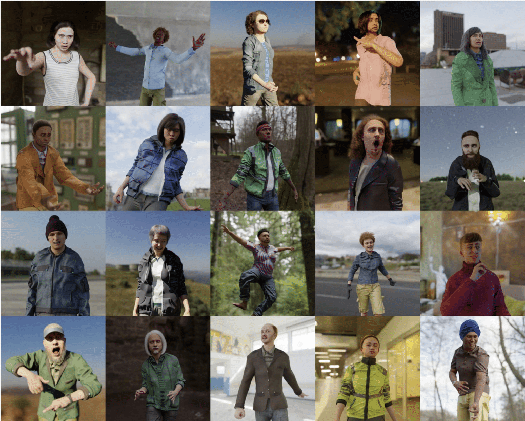
Procedural Humans for Computer Vision