


Understanding VGG16: Concepts, Architecture, and Performance
What Is VGG16?
VGG16 refers to the VGG model, also called VGGNet. It is a convolution neural network (CNN) model supporting 16 layers. K. Simonyan and A. Zisserman from Oxford University proposed this model and published it in a paper called Very Deep Convolutional Networks for Large-Scale Image Recognition.
The VGG16 model can achieve a test accuracy of 92.7% in ImageNet, a dataset containing more than 14 million training images across 1000 object classes. It is one of the top models from the ILSVRC-2014 competition.
VGG16 improves on AlexNet and replaces the large filters with sequences of smaller 3×3 filters. In AlexNet, the kernel size is 11 for the first convolutional layer and 5 for the second layer. The researchers trained the VGG model for several weeks using NVIDIA Titan Black GPUs.
In This Article
The Motivation Behind the VGG Model
Andrew Zisserman and Karen Simonyan first proposed the VGG model in 2013 and created a prototype for the 2014 ImageNet Challenge. They belonged to the Visual Geometry Group (VGG) at Oxford.
This model differed from previous high-performing models in several ways. First, it used a tiny 3×3 receptive field with a 1-pixel stride—for comparison, AlexNet used an 11×11 receptive field with a 4-pixel stride. The 3×3 filters combine to provide the function of a larger receptive field.
The benefit of using multiple smaller layers rather than a single large layer is that more non-linear activation layers accompany the convolution layers, improving the decision functions and allowing the network to converge quickly.
Second, VGG uses a smaller convolutional filter, which reduces the network’s tendency to over-fit during training exercises. A 3×3 filter is the optimal size because a smaller size cannot capture left-right and up-down information. Thus, VGG is the smallest possible model to understand an image’s spatial features. Consistent 3×3 convolutions make the network easy to manage.
VGG16 Architecture
VGG16, as its name suggests, is a 16-layer deep neural network. VGG16 is thus a relatively extensive network with a total of 138 million parameters—it’s huge even by today’s standards. However, the simplicity of the VGGNet16 architecture is its main attraction.
The VGGNet architecture incorporates the most important convolution neural network features.
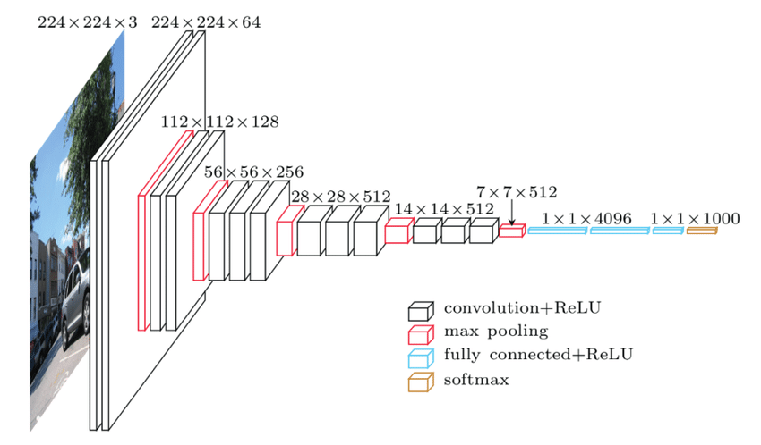
Source: ResearchGate
A VGG network consists of small convolution filters. VGG16 has three fully connected layers and 13 convolutional layers.
Here is a quick outline of the VGG architecture:
- Input—VGGNet receives a 224×224 image input. In the ImageNet competition, the model’s creators kept the image input size constant by cropping a 224×224 section from the center of each image.
- Convolutional layers—the convolutional filters of VGG use the smallest possible receptive field of 3×3. VGG also uses a 1×1 convolution filter as the input’s linear transformation.
- ReLu activation—next is the Rectified Linear Unit Activation Function (ReLU) component, AlexNet’s major innovation for reducing training time. ReLU is a linear function that provides a matching output for positive inputs and outputs zero for negative inputs. VGG has a set convolution stride of 1 pixel to preserve the spatial resolution after convolution (the stride value reflects how many pixels the filter “moves” to cover the entire space of the image).
- Hidden layers—all the VGG network’s hidden layers use ReLU instead of Local Response Normalization like AlexNet. The latter increases training time and memory consumption with little improvement to overall accuracy.
- Pooling layers–A pooling layer follows several convolutional layers—this helps reduce the dimensionality and the number of parameters of the feature maps created by each convolution step. Pooling is crucial given the rapid growth of the number of available filters from 64 to 128, 256, and eventually 512 in the final layers.
- Fully connected layers—VGGNet includes three fully connected layers. The first two layers each have 4096 channels, and the third layer has 1000 channels, one for every class.
VGG16 vs. ResNet
VGG introduced the concept of increasing the number of layers to improve accuracy. However, increasing the number of layers above 20 could prevent the model from converging. The main reason is the vanishing gradient problem—after too many folds, the learning rate is so low that the model’s weights cannot change.
Another issue is gradient explosion. A solution is gradient clipping, which involves “clipping” the error derivative to a certain threshold during backward propagation, and using these clipped gradients to update the weights. When the error derivative is rescaled, weights are also rescaled, and this reduces the chance of an overflow or underflow that can lead to gradient explosion..
The Residual Network (ResNet) architecture uses the concept of skip connections, allowing inputs to “skip” some convolutional layers. The result is a significant reduction in training time and improved accuracy. After the model learns a given feature, it won’t attempt to learn it again—instead, it will focus on learning the new features. It’s a clever approach that can significantly improve model training.
Related content: Read our guide to ResNet
VGG Configuration, Training, and Results
There are five configurations of the VGG network, from A to E. The configuration’s depth increases from A to B, each with more added layers. The following table describes all possible network architectures.
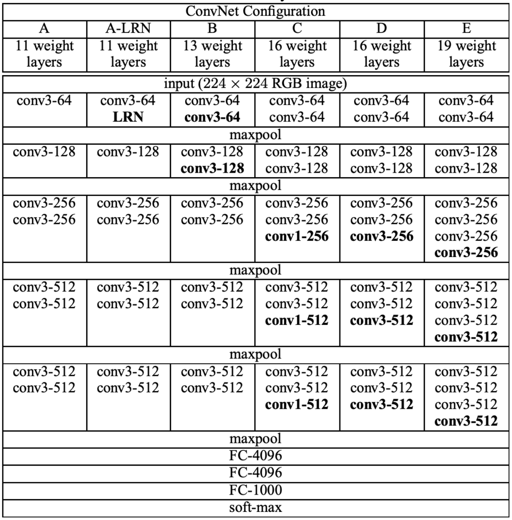
Source for this and the following images: Simonyan and Zisserman, Arxiv.org
Every configuration follows a common architectural pattern, differing only in depth. Network A has 11 weight layers (8 convolutional layers and 3 fully connected layers), while network E has 19 weight layers (16 convolutional layers and 3 fully connected layers).
There are few convolutional layer channels—the number ranges from 64 channels in the first layer to 512 in the last layer (it increases by a factor of two for every max-pooling layer). The figure below shows the total number of parameters in millions.

The process of training VGG is similar to that of AlexNet (Krizhevsky et al.). They both involve optimizing a multinomial logistic regression function to achieve backpropagation. VGG uses mini-batches to avoid a vanishing gradient that arises due to the depth of the network.
During training, the batch size was set to be 256, while the momentum was set to be 0.9. The VGG model introduced dropout regularization in two of the fully connected layers, with the dropout ratio set to 0.5. The network’s initial learning rate was 0.001. When the accuracy of the validation set stopped improving, the learning rate decreased by a factor of 10. The learning rate dropped three times, and training ended after 74 epochs (370,000 iterations).
It took 2-3 weeks to train a VGG network using 4 NVIDIA Titan Black GPUs on the ILSVRC dataset on 1.3 million training images.
The VGG16 network far outperformed previous models in the ILSVRC-2012 and 2013 competitions in an image classification task. The VGG16 architecture achieved the best results in terms of single net performance (7.0% test error). The table below shows the error rates.
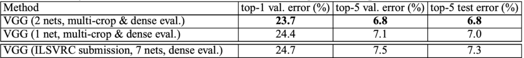
The two main drawbacks of using VGG are its long training time and large model size of 500MB. Modern architectures use skip connections and inceptions to reduce the number of trainable parameters, improving both accuracy and training time.
Read More
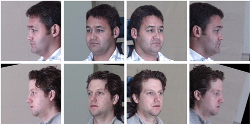
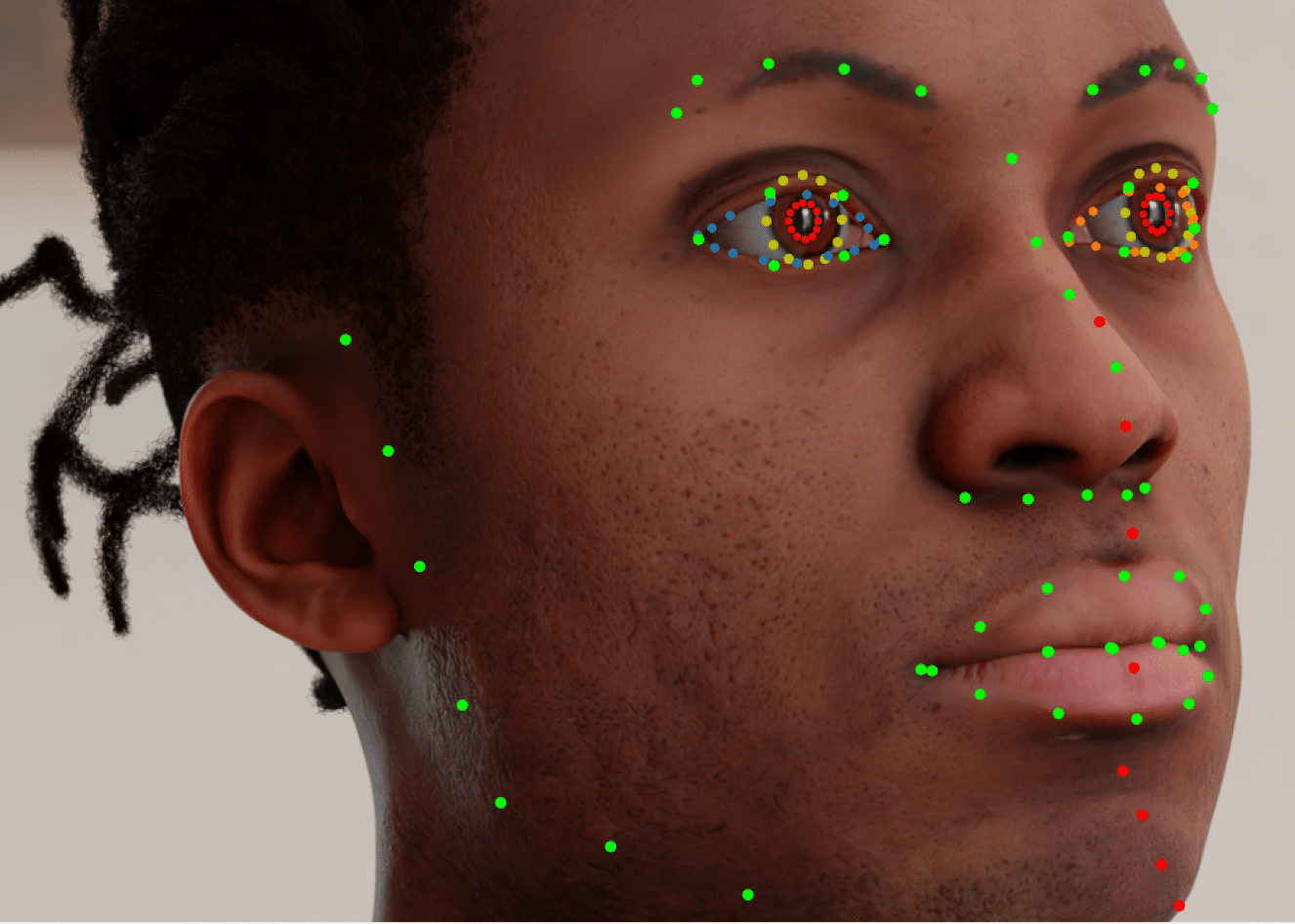
The State of Facial Recognition Today
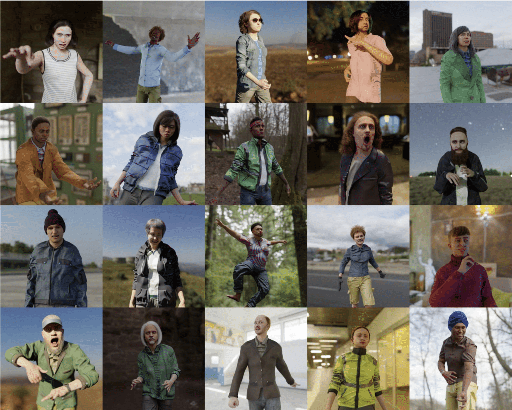
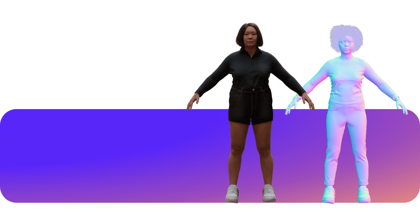
Procedural Humans for Computer Vision